A powerful tool for investigating the inherent structure in the indicators’ set
Multivariate analysis can be helpful in assessing the suitability of the dataset and providing an understanding of the implications of the methodological choices (e.g. weighting, aggregation) during the development of a composite indicator. In the analysis, the statistical information inherent in the indicators’ set can be dealt with grouping information along the two dimensions of the dataset, i.e. along indicators and along constituencies (e.g. countries, regions, sectors, etc.), not independently of each other.
Techniques commonly used in this type of analysis include:
Factor Analysis and Reliability/Item Analysis (e.g. Coefficient Cronbach Alpha) can be used to group the information on the indicators. The aim is to explore whether the different dimensions of the phenomenon are statistically well balanced in the composite indicator. The higher the correlation between the indicators, the fewer statistical dimensions will be present in the dataset. However, if the statistical dimensions do not coincide with the theoretical dimensions of the dataset, then a revision of the set of the sub-indicators might be considered.
Depending on a school of thought, one may see a high correlation among indicators as something to correct for, e.g. by making the weight for a given indicator inversely proportional to the arithmetic mean of the coefficients of determination for each correlation that includes the given indicator. On the other hand, practitioners of multi-criteria decision analysis would tend to consider the existence of correlations as a feature of the problem, not to be corrected for, as correlated indicators may indeed reflect non-compensable different aspects of the problem.
Cluster Analysis can be applied to group the information on constituencies (e.g. countries) in terms of their similarity with respect to the different indicators. This type of analysis can serve multiple purposes, and it can be seen as:
- a purely statistical method of aggregation of indicators,
- a diagnostic tool for assessing the impact of the methodological choices made during the development of the composite indicator,
- a method of disseminating the information on the composite indicator, without losing the information on the dimensions of the indicators,
- a method for selecting groups of countries to impute missing data with a view to decrease the variance of the imputed values.
1. Principal Components Analysis/Factor Analysis
The goal of the Principal Components Analysis (PCA) is to reveal how different variables change in relation to each other, or how they are associated. This is achieved by transforming correlated original variables into a new set of uncorrelated underlying variables (termed principal components) using the covariance matrix, or its standardized form – the correlation matrix. The lack of correlation in the principal components is a useful property because it means that the principal components are measuring different “statistical dimensions” in the data. The new variables are linear combinations of the original ones and are sorted into descending order according to the amount of variance that they account for in the original set of variables. Each new variable accounts for as much of the remaining total variance of the original data as possible. Cumulatively, all the new variables account for 100% of the variation. PCA involves calculating the eigenvalues and their corresponding eigenvectors of the covariance matrix or correlation matrix. Each eigenvalue represents the total remaining variance that the corresponding new variable accounts for. The elements of the eigenvector are the coefficients (loadings) used in the linear transformation of the original variables into the new variables. The expectation from conducting PCA is that correlations among original variables are large enough so that the first few new variables or principal components account for most of the variance. If this holds, no essential insight is lost by further analysis or decision making, and parsimony and clarity in the structure of the relationships are achieved.
Factor analysis (FA) has similar aims to PCA. The basic idea is still that it may be possible to describe a set of variables in terms of a smaller number of factors, and hence elucidate the relationship between these variables. There is however, one important difference: PCA is not based on any particular statistical model, but FA is based on a rather special model. There are several approaches in Factor analysis, e.g. communalities, maximum likelihood factors, centroid method, principal axis method, etc. The most common is the use of PCA to extract the first m principal components and consider them as factors and neglect the remaining. On the issue of how factors should be retained in the analysis without losing too much information methodologists’ opinions differ. The decision of when to stop extracting factors basically depends on when there is only very little "random" variability left, and it is rather arbitrary. However, various guidelines (“stopping rules”) have been developed, such as the Kaiser criterion, the scree plot, variance explained criteria, the Joliffe criterion etc. After choosing the number of factors to keep, rotation is a standard step performed to enhance the interpretability of the results. There are various rotational strategies that have been proposed. The goal of all of these strategies is to obtain a clear pattern of loadings. However, different rotations imply different loadings, and thus different meanings of principal components - a problem some cite as a drawback to the method. The most common rotation method is the “varimax rotation”.
2. Cronbach Coefficient Alpha
Another way to investigate the degree of the correlations among a set of variables is to use the Cronbach Coefficient Alpha. This statistic is the most common estimate of internal consistency of items in a model or survey – Reliability/Item Analysis. It assesses how well a set of items (in our terminology indicators) measures a single unidimensional object (e.g. attitude, phenomenon etc.).
Cronbach's Coefficient Alpha can be defined as:
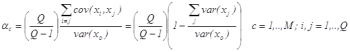
where M as usual indicates the number of countries considered, Q the number of sub-indicators available, and

is the sum of all indicators.
Cronbach Coefficient Alpha measures the portion of total variability of the sample of indicators due to the correlation of indicators. It grows with the number of indicators and with the covariance of each pair of them. If no correlation exists and indicators are independent then Cronbach Coefficient Alpha is equal to zero, while if indicators are perfectly correlated the Cronbach Coefficient Alpha is equal to one. Cronbach Coefficient Alpha is not a statistical test but a coefficient of reliability based on the correlations between indicators: a high value could imply that the indicators are measuring the same underlying construct. Though widely interpreted as such, strictly speaking Cronbach Coefficient Alpha is not a measure of unidimensionality. A set of indicators can have a high alpha and still be multidimensional. This happens when there are separate clusters of sub-indicators (separate dimensions) which inter-correlate highly, even though the clusters themselves are not highly correlated. An issue is how large the Cronbach Coefficient Alpha must be. Some authors suggest 0.7 as an acceptable reliability threshold, while others are as lenient as 0.60. In general this varies by discipline.
3. Cluster Analysis
Cluster analysis is the name given to a collection of algorithms used to classify objects, e.g. countries, species, individuals. The classification has the aim of reducing the dimensionality of a dataset by exploiting the similarities/dissimilarities between cases. The result will be a set of clusters such that cases within a cluster are more similar to each other than they are to cases in other clusters. Cluster analysis has been applied in a wide variety of research problems, from medicine and psychiatry to archaeology. In general whenever one needs to classify a large amount of information into manageable meaningful piles, or discover similarities between objects, cluster analysis is of great utility.
Cluster analysis techniques can be hierarchical (for example the tree clustering), i.e. the resultant classification has a increasing number of nested classes, or non-hierarchical when the number of clusters is decided ex ante (for example the k-means clustering). Care should be taken that groups (classes) are meaningful in some fashion and are not arbitrary or artificial. To do so the clustering techniques attempt to have more in common with own group than with other groups, through minimization of internal variation while maximizing variation between groups.
Homogeneous and distinct groups are delineated based upon assessment of distances or in the case of Ward's method, an F-test. A distance measure is an appraisal of the degree of similarity or dissimilarity between cases in the set. A small distance is equivalent to a large similarity. It can be based on a single dimension or on multiple dimensions, for example countries can be evaluated according to the composite indicator or they can be evaluated according to all single indicators. Notice that Cluster analysis does not “care” whether the distances are real (as in the case of quantitative indicators) or given by the researcher on the basis of an ordinal ranking of alternatives (as in the case of qualitative indicators). Some of the most common distance measures include Euclidean and non-Euclidean distances (e.g. city-block). One problem with Euclidean distances is that they can be greatly influenced by variables that have the largest values. One way around this problem is to standardise the variables.
Having decided how to measure similarity (the distance measure), the next step is to choose the clustering algorithm, i.e. the rules which govern how distances are measured between clusters. There are many methods available, the criteria used differ and hence different classifications may be obtained for the same data, even using the same distance measure. The most common linkage rules are: single linkage (nearest neighbor), complete linkage (furthest neighbor), unweighted pair-group average, weighted pair-group average, Ward’s method.
Examples of composite indicators that have used the methods above:
| Method | Composite indicators |
|---|---|
| Principal Componenets Analysis/Factor analysis | Environmental Sustainability Index General Indicator of Science & Technology Internal Market Index Business Climate Indicator Success of software process implementation |
| Cronbach Coefficient Alpha | Success of software process implementation Compassion Fatigue following the Sep. 11 Terrorist Attacks |
| Cluster Analysis | Index of healthy conditions Composite Indicator of a Firm’s Innovativeness |
Next
| Originally Published | Last Updated | 21 Apr 2018 | 27 Mar 2025 |
| Knowledge service | Metadata | Composite Indicators |